Moving and adapting

This is an example of how to move the interface and adapt the mesh.

We implement the finite volume moving mesh method presented in [CMR+18].

CMR+18

3. Chalons, J. Magiera, C. Rohde, M. Wiebe. A Finite-Volume Tracking Scheme for Two-Phase Compressible Flow. Theory, Numerics and Applications of Hyperbolic Problems I, pp. 309–322, 2018.

Grid creation

We use the vertical grid file that contains an interface \(\Gamma = {0.5} \times [0, 1]\) embedded in a domain \(\Omega = [0,1]^2\). For this example, we have to construct an adaptive leaf grid view and we will need to obtain the hierarchical grid object.

from dune.grid import reader
from dune.mmesh import mmesh
from dune.fem.view import adaptiveLeafGridView as adaptive
dim = 2
file = "grids/vertical.msh"
gridView = adaptive( mmesh((reader.gmsh, file), dim) )
hgrid = gridView.hierarchicalGrid
igridView = hgrid.interfaceGrid

Problem

Let us consider the following transport problem. \begin{align} u_t + \operatorname{div} f(u) = 0, & \qquad \text{in } \Omega \times [0,T], \\ u(\cdot, 0) = u_0, & \qquad \text{in } \Omega \end{align} where \begin{align} f(u) &= [1,0]^T u, \\ u_0(x,y) &= (0.5+x) \chi_{x<0.5}. \end{align}

Further, the interface is supposed to move with the transport speed in \(f\), i.e. \(m = [1,0]^T\). \begin{align*} \renewcommand{\jump}[1]{[\mskip-5mu[ #1 ]\mskip-5mu]} \end{align*}

from ufl import *
from dune.ufl import Constant

t = 0
tEnd = 0.4
dt = 0.04

def speed():
    return as_vector([1.0, 0.0])

def movement(x):
    return as_vector([1.0, 0.0])

def f(u):
    return speed() * u

def u0(x):
    return conditional(x[0] < 0.5, 0.5+x[0], 0.0)

def uexact(x, t):
    return u0( x - t * speed() )

Finite Volume Moving Mesh Method

We use a Finite Volume Moving Mesh method to keep the discontinuity sharp. It can be formulated by \begin{align} \int_\Omega (u^{n+1} |det(\Psi)| - u^n) v\ dx + \Delta t \int_\mathcal{F} \big( g(u^{n+1}, n) - h(u^{n+1}, n) \big) \jump{v}\ dS = 0 \end{align} where \(\Psi := x + \Delta t s\) and s is a linear interpolation of the interface’s vertex movement m on the bulk triangulation.

The numerical fluxes \(g(u, n)\) and \(h(u, n)\) are assumed to be consistent with the flux functions \(f(u) \cdot n\) and \(u s \cdot n\), respectively.

from dune.fem.space import finiteVolume

space = finiteVolume(gridView)
u = TrialFunction(space)
v = TestFunction(space)

x = SpatialCoordinate(space)
n = FacetNormal(space)

uh = space.interpolate(u0(x), name="uh")
uh_old = uh.copy()

import numpy as np
from dune.geometry import vertex
from dune.mmesh import edgeMovement

def getShifts():
    mapper = igridView.mapper({vertex: 1})
    shifts = np.zeros((mapper.size, dim))
    for v in igridView.vertices:
        shifts[ mapper.index(v) ] = as_vector(movement( v.geometry.center ))
    return shifts

em = edgeMovement(gridView, getShifts())
time = Constant(t, name="time")

def g(u, n):
    sgn = inner(speed(), n('+'))
    return inner( conditional( sgn > 0, f( u('+') ), f( u('-') ) ), n('+') )

def gBnd(u, n):
    sgn = inner(speed(), n)
    return inner( conditional( sgn > 0, f(u), f(uexact(x, time)) ), n )

def h(u, n):
    sgn = inner(em('+'), n('+'))
    return conditional( sgn > 0, sgn * u('+'), sgn * u('-') )

from dune.fem.scheme import galerkin

tau = Constant(dt, name="tau")
detPsi = abs(det(nabla_grad(x + tau * em)))

a = (u * detPsi - uh_old) * v * dx
a += tau * (g(u, n) - h(u, n)) * jump(v) * dS
a += tau * gBnd(u, n) * v * ds

scheme = galerkin([a == 0], solver=("suitesparse","umfpack"))

Timeloop

We need to set the "fem.adaptation.method" parameter to "callback" in order to use the non-hierarchical adaptation strategy of Dune-MMesh. Then, within the time loop, we can adapt the mesh according to the following strategy.

from dune.fem import parameter, adapt
parameter.append( { "fem.adaptation.method": "callback" } )
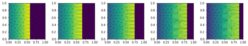
from dune.fem.plotting import plotPointData as plot
import matplotlib.pyplot as plt
fig, axs = plt.subplots(1, 5, figsize=(12,3))

i = 0
while t < tEnd:
    hgrid.markElements()
    hgrid.ensureInterfaceMovement(getShifts()*dt)
    adapt([uh])

    hgrid.moveInterface(getShifts()*dt)

    em.assign(edgeMovement(gridView, getShifts()))
    t += dt
    time.assign(t)

    uh_old.assign(uh)
    scheme.solve(target=uh)

    i += 1
    if i % 2 == 0:
        plot(uh, figure=(fig, axs[i//2-1]), clim=[0,1], colorbar=None)